Paper
Butcher, Jasper, et al. "De novo design of all-atom biomolecular interactions with rfdiffusion3." bioRxiv (2025).
De novo Design of All-atom Biomolecular Interactions with RFdiffusion3 | bioRxiv
Github
Abstract
Deep learning has accelerated protein design, but most existing methods are restricted to generating protein backbone coordinates and often neglect interactions with other biomolecules. We present RFdiffusion3 (RFD3), a diffusion model that generates protein structures in the context of ligands, nucleic acids and other non-protein constellations of atoms. Because all polymer atoms are modeled explicitly, conditioning the model on complex sets of atom-level constraints for enzyme design and other challenges is both simpler and more effective than previous approaches. RFD3 achieves improved performance compared to prior approaches on a range of in silico benchmarks with one tenth the computational cost. Finally, we demon strate the broad applicability of RFD3 by designing and experimentally characterizing DNA binding proteins and cysteine hydrolases. The ability to rapidly generate protein structures guided by complex sets of atom-level constraints in the context of arbitrary non-protein atoms should further expand the range of functions attainable through protein design.
[Problem]
- 기존 딥러닝 기반 단백질 design은 residue-level에서 작동하기 때문에, small molecule이나 핵산같은 비단백질 원자와의 구체적인 sidechain interaction을 설계할 수 없다.
[Solution]
- RFD3는 모든 원자를 모델링해서 효소 설계에 필요한 atom level에서의 제약 조건을 지정할 수 있게 한다. 이전 방법들과 달리 복잡한 우회 방식이 필요하지 않다.
[Contribution]
- 성능 향상 및 계산 비용 절감을 동시에 달성했다. 10배 빠른 속도는 대규모 스크리닝이나 반복적인 설계 최적화에 큰 장점이 된다.
Motivation
| Model | Representations | Limitations |
| RFD1 | amino-acid level | protein monomer, assembly, protein-protein bind 설계는 가능하지만 small molecules나 nucleic acids과의 특정 side chain interaction 설계 불가능 |
| BindCraft | amino-acid level | RFD1과 동일 |
| RFD2 | residue level + additional side chain atom | catalytic이나 ligand binding에 중요한 일부 side chain atom만 conditioning 가능하지만 diffusion 자체는 여전히 residue level |
| AF3 | all atom | 설계용이 아니고 pairformer 모듈이 시간, 연산 비용 증가 |
Concept
[1] Diffusion Model
- Diffusion은 데이터에 점진적으로 noise를 추가하는 forward process와 노이즈로부터 원본 데이터를 복원하는 reverse process로 구성된다.
RFD3에서는
- Forward process: protein의 atom 좌표에 가우시안 노이즈를 점진적으로 추가
- Reverse process (denoising): 노이즈가 추가된 좌표로부터 원래 구조를 예측

- 논문에서는 그림처럼 100 step의 diffusion trajectory를 사용한다. ($t$ = 100)
[2] 14-Atom Residue Representation
핵심: seqeunce가 알려지지 않은 상태에서 sidechain을 어떻게 표현할까?
모든 아미노산을 4개의 backbone atom + 10개의 side chain atom으로 통일해서 표현한다.
왜 10개인가? 가장 큰 sidechain을 가지고 있는 트립토판(Tryptophan)이 10개의 sidechain atom을 가지기 때문이다.
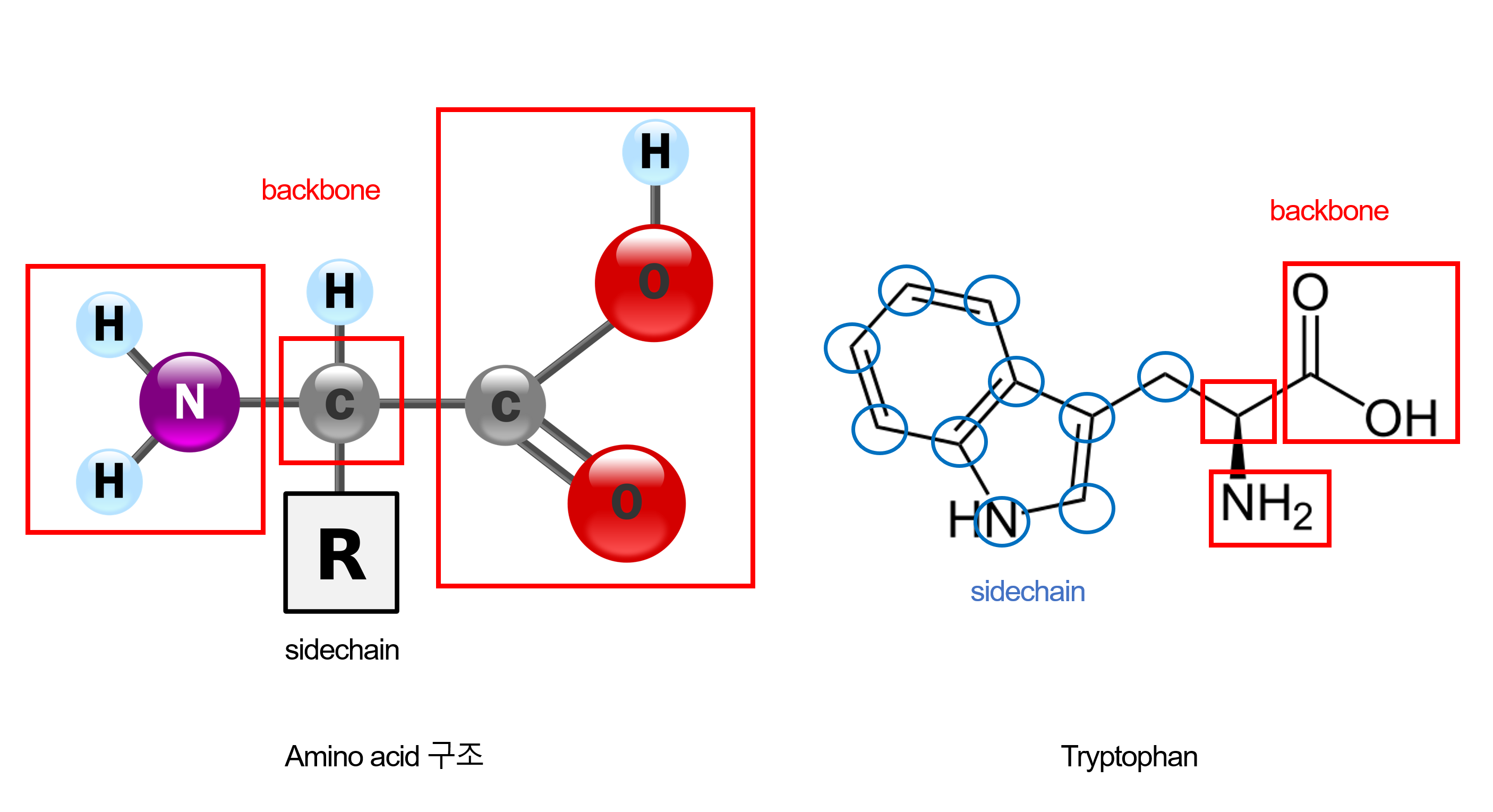
[추가] Tryptophan이 왜 10개의 sidechain atom을 가지는지 간단하게 보충 설명,
- 아미노산은 왼쪽처럼 backbone과 sidechain으로 이루어져 있다.
- 그리고 단백질 구조 분석에서는 heavy atom을 기준으로 세는 것이 표준이다. (H을 제외해서 C, N, O, S 등을 세면 된다.)
- 여기서 우리가 Tryptophan의 sidechain의 atom 개수를 세기 위해서는 backbone을 제외해야 한다.
- 오른쪽 그림처럼 backbone을 제외한 파랑색 원의 개수를 세면 10개가 나온다.

- Tryptophan는 10개로 표현,그렇다면 더 작은 sidechain을 가진 아미노산은 어떻게 채울까?
- 작은 side chain을 가진 아미노산: 사용하지 않는 원자들은 Cβ 위치에 virtual atom으로 배치 (Glycine의 경우 Cα에만, Cβ가 없기 때문에)
ccd_ordering_atomchar = {
    'TRP': (" N  "," CA "," C  "," O  "," CB "," CG "," CD1"," CD2"," NE1"," CE2"," CE3"," CZ2"," CZ3"," CH2"),  # trp
    'HIS': (" N  "," CA "," C  "," O  "," CB "," CG "," ND1"," CD2"," CE1"," NE2",  None,  None,  None,  None),  # his
    'TYR': (" N  "," CA "," C  "," O  "," CB "," CG "," CD1"," CD2"," CE1"," CE2"," CZ "," OH ",  None,  None),  # tyr
    'PHE': (" N  "," CA "," C  "," O  "," CB "," CG "," CD1"," CD2"," CE1"," CE2"," CZ ",  None,  None,  None),  # phe
    'ASN': (" N  "," CA "," C  "," O  "," CB "," CG "," OD1"," ND2",  None,  None,  None,  None,  None,  None),  # asn
    'ASP': (" N  "," CA "," C  "," O  "," CB "," CG "," OD1"," OD2",  None,  None,  None,  None,  None,  None),  # asp
    'GLN': (" N  "," CA "," C  "," O  "," CB "," CG "," CD "," OE1"," NE2",  None,  None,  None,  None,  None),  # gln
    'GLU': (" N  "," CA "," C  "," O  "," CB "," CG "," CD "," OE1"," OE2",  None,  None,  None,  None,  None),  # glu
    'CYS': (" N  "," CA "," C  "," O  "," CB "," SG ",  None,  None,  None,  None,  None,  None,  None,  None),  # cys
    'SER': (" N  "," CA "," C  "," O  "," CB "," OG ",  None,  None,  None,  None,  None,  None,  None,  None),  # ser
    'THR': (" N  "," CA "," C  "," O  "," CB "," OG1"," CG2",  None,  None,  None,  None,  None,  None,  None),  # thr
    'LEU': (" N  "," CA "," C  "," O  "," CB "," CG "," CD1"," CD2",  None,  None,  None,  None,  None,  None),  # leu
    'VAL': (" N  "," CA "," C  "," O  "," CB "," CG1"," CG2",  None,  None,  None,  None,  None,  None,  None),  # val
    'ILE': (" N  "," CA "," C  "," O  "," CB "," CG1"," CG2"," CD1",  None,  None,  None,  None,  None,  None),  # ile
    'MET': (" N  "," CA "," C  "," O  "," CB "," CG "," SD "," CE ",  None,  None,  None,  None,  None,  None),  # met
    'LYS': (" N  "," CA "," C  "," O  "," CB "," CG "," CD "," CE "," NZ ",  None,  None,  None,  None,  None),  # lys
    'ARG': (" N  "," CA "," C  "," O  "," CB "," CG "," CD "," NE "," CZ "," NH1"," NH2",  None,  None,  None),  # arg
    'PRO': (" N  "," CA "," C  "," O  "," CB "," CG "," CD ",  None,  None,  None,  None,  None,  None,  None),  # pro
    'ALA': (" N  "," CA "," C  "," O  "," CB ",  None,  None,  None,  None,  None,  None,  None,  None,  None),  # ala
    'GLY': (" N  "," CA "," C  "," O  ",  None,  None,  None,  None,  None,  None,  None,  None,  None,  None),  # gly
    'UNK': (" N  "," CA "," C  "," O  "," CB ",  None,  None,  None,  None,  None,  None,  None,  None,  None),  # unk
    'MSK': (" N  "," CA "," C  "," O  "," CB ",  None,  None,  None,  None,  None,  None,  None,  None,  None),  # mask
}- Serine의 말단 산소와 Cysteine의 황은 서로 다른 virtual atom으로 표현되어 구분 가능
[3] Atom-level hydrogen bond conditioning
- Classifier-Free Guidance (CFG): 이미지 diffusion 분야에서 개발된 기법으로, conditioning 정보에 대한 모델의 adherence를 향상시킨다 (Ho, Jonathan, and Tim Salimans. "Classifier-free diffusion guidance." arXiv preprint arXiv:2207.12598 (2022).)
- use_classifier_free_guidance: False (Inference)
작동 방식: 각 denoising step에서 두 번의 forward pass 수행:
- Conditioning 정보를 사용한 예측
- Conditioning 없이 (unconditional) 예측
- 두 예측의 가중 평균으로 최종 출력 결정
[4] 용어 정의
1. Hotspot
- 기존 모델들은 Residue level에서 hotspot을 지정했다면, RFD3는 atom level로도 가능하다.
2. Residue island
- 서열상으로는 떨어져 있지만, 3차원 구조에서 특정 기능을 수행하기 위해 모여 있는 연속적인 resiude stretch의 개수
- 개수가 많아질수록 모두 포함하면서 안정적인 protein scaffold 만들기가 어려워진다.
3. RASA (Relative Accessible Surface Area)
- 원자가 solvent(물 등)에 노출된 상대적인 면적
- Ligand 설계 시 특정 원자가 protein 내부에 얼마나 깊이 박혀야(burial) 하는지 지시하는 condition
4. Tip atoms
- Amino acid sidechain 끝에 위치하여 실제 반응이나 결합에 참여하는 핵심 atom들
Soultion
[Overview] Model architecture

0. AlphaFold3: Transformer-based U-Net Architecture
AF3의 diffusion module과 유사한 구조를 가졌지만, 설계 목적에 맞게 경량화했다.
AF3는 sequence 정보를 처리하기 위해 무거운 pairformer(48 layers)가 필요하다. 하지만 설계에서는 seq가 입력이 아니므로 경량화가 가능하다.
1. Input
| Category | Shape | Details |
| X_noisy_L | [N_atoms, 3] | 노이즈가 추가된 원자 좌표 |
| t (timestep) | scalar → Fourier embedding | 현재 diffusion 진행 상태 |
| Token features | [N_tokens, d_token] | residue 단위 |
| Atom features | [N_tokens × 14, d_atom] | atom 단위 |
| Masks | various | motif/atom, padding 등 |
2. Token features
Shape: [N_tokens, d_token]
| Feature | Dim | Details | Example |
| restype | 32 | 아미노산 종류 one-hot encoding | ALA=[1,0,0,...] |
| ref_motif_token_type | 3 | motif 3 types: - Diffuse(새로 생성할 residue) - Indexed motif (위치 고정 residue) - Unindexed motif (구조 알지만 서열 위치 모르는 residue) |
[1,0,0], [0,1,0], [0,0,1] |
| ref_plddt | 1 | 구조 신뢰도 | +1(높음), -1(낮음), 0(모름) |
| is_non_loopy | 1 | 2차 구조 옵션 | +1(helix,sheet), -1(loop), 0(지정X) |
3. Atom features
Shape: [N_tokens × 14, d_atom]
| Feature | D | Details | Example |
| ref_atom_name_chars | 256 | [atom] atom name encoding (4 x 64 classes) | N [N, _, _, _], CA [C, A, _, _] |
| ref_element | 128 | [atom] 원소 번호 기반 one-hot (128 classes) | C - 원자번호 6 [0,0,...1,0,...] |
| ref_charge | 1 | [atom] 형식 전하 | -1, 0, +1 |
| ref_mask | 1 | [atom] real atom, virtual atom | 1, 0 |
| ref_pos | 3 | [atom] (x, y, z) | [12.5, 8.3, -4.2] |
| ref_is_motif_atom_wtih_fixed_coord | 1 | [motif] 좌표가 고정된 atom | 1=고정, 0=diffuse |
| ref_is_motif_atom_unindexed | 1 | [motif] unindexed motif atom | 1=unindexed |
| has_zero_occupancy | 1 | [motif] occupancy 0 atom (무시할 원자) | 1=무시 |
| ref_atomwise_rasa | 3 | [conditioning] surface 노출도 one-hot | buried, partial, exposed |
| active_donor | 1 | [conditioning] H-bond donor | 1=donor |
| active_acceptor | 1 | [conditioning] H-bond acceptor | 1=acceptor |
| is_atom_level_hotspot | 1 | [conditioning] PPI hotspot | 1=hotspot |
4. Feature initializer (2 blocks)
| Category | Details |
| input | Token Features + Atom Features |
| output | 아래 표 참고 |
| role | 모든 representation 초기화, Global (Pairformer ×2) |
→ "We thus shrunk the Pairformer from 48 to just 2 layers" (설계 모델에서는 seq가 아닌 conditioning 정보만 처리하면 되므로 2 layers로 경량화하는 것이 가능)
# Pairformer
| Model | Pairformer layers | Total parameters |
| AF3 | 48 | ~350M |
| RFD3 | 2 | 168M |
※ Output (Step1: init_tokens → Step2: init_atoms)
| Output | Level | Shape | Details |
| S_I | Token | [N_tokens, 384] | residue |
| Z_II | Toekn pair | [N_tokens, N_tokens, 128] | residue pair |
| Q_L | Atom | [N_atoms, 128] | atom |
| C_L | Atom | [N_atoms, 128] | atom conditioning (t 포함) |
| P_LL | Atom pair | [N_atoms, N_atoms, 16] | atom pair |
5. [Encoder] Atom encoder (3 blocks)
| Category | Details |
| input | Q_L (atom repr) + C_L (conditioning) + P_LL (atom pair) |
| output | Q_L (updated atom feature) |
| role | 원자 수준 정보 처리, local 구조 패턴 추출, sparse (가까운 128개 atom만) |
Sparse attention
일반 attention은 모든 atom pair 계산, RFD3는 가까운 128개 atom만
6. [Encoder] Downcast (Atom → Token)
| Category | Details |
| input | Q_L (atom feature) + A_I (기존 token feature) |
| output | A_I (updated token feature) |
| role | Cross-attention weighted sum |
[14개 atom feature] → attention weighted sum → [1개 token feature]
단순 평균이 아닌 이유? 모든 atom이 동일하게 중요하지 않다.
7. [Encoder] Token Transformer (18 blocks)
| Category | Details |
| input | A_I + S_I + Z_II |
| output | A_I (updated) |
| role | Residue 수준 local 정보 교환, Sparse (sequence 이웃 8개 + 거리 기반 32개) |
8. [Decoder] Upcast (Token → Atom)
| Category | Details |
| input | Q_L (atom feature) + A_I (token feature) |
| output | Q_L (updated atom feature) |
| role | Cross-attention |
[1개 token feature] → cross-attention → [14개 atom feature]
Query: Q_L (14개 원자)
Key/Value: A_I (1개 토큰)
9. [Decoder] Atom decoder (3 blocks)
| Category | Details |
| input | Q_L + C_L (conditioning) + P_LL (atom pair) |
| output | Q_L (refined atom feature) |
| role | 원자 수준 정보 정제, Sparse attention (가까운 128개 atom) |
※ 8-9는 3회 반복: Upcast → Atom Decoder → Upcast → Atom Decoder → Upcast → Atom Decoder
10. [Decoder] Output heads
| Head | Input | Output | Shape |
| to_r_update | Q_L | X_denoised (좌표) | [N_atoms, 3] |
| sequence_head | A_I | sequence_logits (서열) | [N_tokens, 32] |
11. Recycling
| Category | Details |
| 범위 | 5~10 |
| 횟수 | 2회 |
| 역할 | Output을 다시 input으로 넣어 accuracy 향상 |
[1] Transformer-based U-Net Architecture
AlphaFold3의 diffusion module과 유사한 구조를 채택하되, 설계 목적에 맞게 경량화했다.
1. Downsampling Module: 부분적으로 노이즈가 추가된 구조를 포함한 atomic/residue 수준 feature 인코딩
2. Sparse Transformer Module:
- Token-wise 정보 처리
- 핵심 차이점: Triangle multiplicative update와 triangle attention을 제거하여 연산 비용 절감
3. Upsampling Module:
- Token-wise feature로 atomic feature를 modulate
- 좌표 업데이트 예측
[2] Atom-Token Feature Exchange
- Backbone과 sidechain 좌표의 joint sampling을 위해 atom-level과 residue-level feature 간의 효과적인 coupling이 필요하다.
1. Distance-based Sparse Attention
- 노이즈 상태에서 기하학적으로 가까운 residue와 atom만 서로 attend
- local interaction (모든 atom과 attention 안 한다는 뜻), overfitting 방지
2. Cross Attention for Up/Down-pooling
- Pagnoni, Artidoro, et al. "Byte latent transformer: Patches scale better than tokens." Proceedings of the 63rd Annual Meeting of the Association for Computational Linguistics (Volume 1: Long Papers). 2025.
- Fine-grained atom representation ↔ Coarser-grained token representation 간 정보 교환
- 각 원자의 feature에 attention 가중치를 적용한 후 token feature로 pooling
- Token splitting을 통한 cross attention으로 token feature를 다시 읽어옴
[3] Conditioning mechanism
1. Atomic Motif Scaffolding

목적: Enzyme 활성 부위 같은 원자 수준 motif를 scaffolding
방법:
- 각 촉매 잔기에 대해 별도의 token을 diffused token에 추가
- 이 motif conditioning token은 고정할 원자들만 포함 (14개 전체가 아님)
- 네트워크가 diffused protein side chain 중 하나를 고정된 원자와 overlap시키도록 학습
RFD2와의 차이
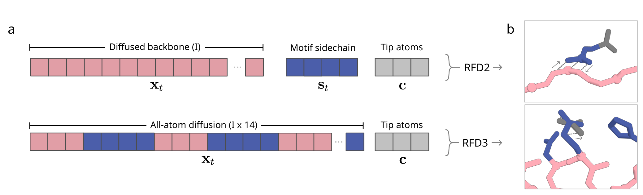
- RFD2: Tip atoms을 명시적으로 토큰화해야 함 (새로운 데이터 타입)
- RFD3: Tip atoms이 다른 모든 토큰과 동일하되 좌표만 고정
2. Protein-DNA Co-diffusion
목적: DNA 결합 단백질 설계 시 DNA 서열만 주어지면 DNA 구조와 단백질 구조를 동시에 생성

접근법:
- DNA 서열이 주어지면 네트워크가 protein 구조와 DNA conformation을 jointly predict
- Bound DNA의 shape를 추론하는 과제를 네트워크에 전달
3. Protein-Ligand Co-diffusion
목적: 리간드 identity만 주어지면 리간드 conformation과 단백질 구조를 동시에 생성

장점:
- 기존 방법은 rigid ligand conformation을 입력으로 요구
- RFD3는 flexible ligand의 여러 conformer를 자동으로 탐색
4. Hydrogen Bond Conditioning

Atom-level hydrogen bond conditioning? (training)
- ligand의 특정 원자가 protein과 수소 결합을 형성하도록 설정 (Donor, Acceptor)
- PDB 구조들 HBPLUS tool로 실제 H-bond 계산 후 filtering (motif랑 diffuse만) - Subsample (50% 확률로 일부만 사용)
- PDB 학습 sample 중 20% conditioning on, 80% conditioning off
- [Result] 논문에서 CFG는 hydrogen bond conditioning의 만족률을 26.67% → 32.67% → 36.67%로 향상시켰다
- DNA bases에 대해서도 유사한 경향: 11% → 11.3% → 12.5%
5. Solvent Accessibility Conditioning

목적: 리간드 원자의 burial 정도 제어
- RASA (Relative Accessible Surface Area) 라벨 제공
- "Buried" 또는 "Exposed"로 지정
- 400개 설계 기준으로 지정된 RASA에 따른 분포가 명확히 분리됨
6. Centre of Mass (COM) Conditioning

목적: 생성되는 단백질의 중심 위치를 타겟 분자나 motif에 대해 상대적으로 지정
방법: 초기화된 noise cloud의 위치로 COM 가이드, OCM conditioning 없이 생성하면 random한 방향에서 target에 접근
Atom feature는 X, 좌표 전처리에 사용
7. Symmetry-constrained Diffusion

목적: 대칭 구조 생성 (C2, C3, C5, C7, D2 등)
방법: Symmetric noise를 입력으로 제공, diffusion step 마다 (초반 90%), 복사/회전
검증 결과 (AF3 Cα RMSD, 여기서 RMSD는 대칭 변환 후 subunit들을 superimpose 했을 때 차이, 낮을수록 대칭):
- D2: 0.832 Å
- C3: 0.450 Å
- C5: 0.614 Å
- C7: 0.539 Å
[4] Training Procedure
1. Training Data
- PDB (Protein Data Bank): 2024년 12월까지 등록된 모든 구조
- AF2 Distillation: Hsu et al.의 AlphaFold2 예측 구조
- Protein-protein, protein-small molecule, protein-DNA interface design, functional motif scaffolding
2. Training method
3. Inference Pipeline
- Step scale η = 1.5
- Noise level γ₀ = 0.6
- Denoising steps: 200
RFD3가 생성한 interface residue를 그대로 유지해도 되는가?
→ 큰 성능 차이 X
Sequence Design:
- 구조 생성 후 ProteinMPNN (단백질 전용) 또는 LigandMPNN (비단백질 원자 포함 시) 사용
- 이유: RFD3는 마지막 diffusion step에서만 최종 backbone 구조를 보므로, 별도 sequence redesign이 구조-서열 일관성 향상
[논문] RFD3 only sees the final backbone structure in the last diffusion step.
→ 문제:
- Network는 diffusion 과정 중에 backbone이 계속 변하는 상황에서 sidechain을 예측
- 마지막 step에서야 backbone이 확정되지만, 그때는 이미 sidechain도 함께 출력됨
- Backbone과 sidechain (sequence)의 joint optimization이 충분히 이루어지지 않음
→ 해결: ProteinMPNN/LigandMPNN Redesign
- ProteinMPNN은 고정된 backbone 구조가 주어졌을 때 최적의 sequence를 예측하는 inverse folding 모델이다.
→ Why 성능 향상?
- ProteinMPNN은 확정된 backbone 전체를 보고 sequence를 결정
- Backbone의 local geometry, burial, secondary structure 등을 고려
- RFD3처럼 noisy intermediate를 거치지 않음
Dauparas, Justas, et al. "Robust deep learning–based protein sequence design using ProteinMPNN." Science 378.6615 (2022): 49-56.

[Motivation]
단백질 서열 설계 문제의 핵심은 주어진 backbone 구조에 대해, 그 구조로 folding될 아미노산 서열을 찾는 것이다.
[ProteinMPNN architecture]
1. Input Features

Baseline model의 input:
- Cα-Cα 원자 간 거리
- 상대적 Cα-Cα-Cα frame orientation 및 rotation
- Backbone dihedral angles
updated input (Experiment 1):
- N, Cα, C, O 원자 간 거리
- Virtual Cβ 위치: 다른 backbone 원자들을 기반으로 계산된 가상의 Cβ 원자
- 이 추가 특징으로 sequence recovery가 41.2% → 49.0%로 향상 (표에 기재되어 있음)
설계 근거: Interatomic distance가 dihedral angle이나 frame orientation보다 residue 간 상호작용을 포착하는 데 더 좋은 inductive bias를 제공한다.
2. Backbone Encoder
구조:
- 3개의 encoder layer
- 128 hidden dimensions
- Node update + Edge update (Experiment 2에서 추가)
Edge update의 효과:
- Experiment 2: Edge update만 추가 시 43.1% sequence recovery
- Experiment 3: Input features + Edge update 결합 시 50.5% sequence recovery
Nearest neighbor 결정:
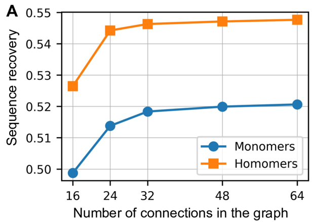
- 테스트한 값: 16, 24, 32, 48, 64 nearest-Cα neighbors
- 최적 범위: 32~48 neighbors에서 성능 포화 (위 그림 참고)
- 설계 근거: 특정 위치의 아미노산 최적성은 주로 immediate protein environment에 의해 결정되므로, locally connected graph neural network로 충분하다.
3. Sequence Decoder with Order-Agnostic Autoregressive Model


기존 방식 (Fixed N→C decoding)의 문제:
- N terminus에서 C terminus로 순차적으로 디코딩
- 앞선 위치의 서열 context를 뒤의 위치가 활용할 수 없음
Order-agnostic decoding의 장점:
- 디코딩 순서를 모든 가능한 permutation에서 무작위로 샘플링
- Sequence recovery: 50.5% → 50.8%로 향상 (3 → 4)
- 서열의 일부가 고정된 경우(예: binder design에서 target 서열이 알려진 경우), 고정된 부분을 먼저 디코딩하고 나머지 위치의 context로 활용 가능
구현 방식:
- 고정된 residue는 디코딩을 skip하고, 나머지 위치의 sequence context에는 포함됨
4. Multichain 및 Symmetry-aware Design
Chain equivariance 구현:
- Per-chain relative positional encoding을 ±32 residues로 제한
- 같은 chain vs 다른 chain 여부를 나타내는 binary feature 추가
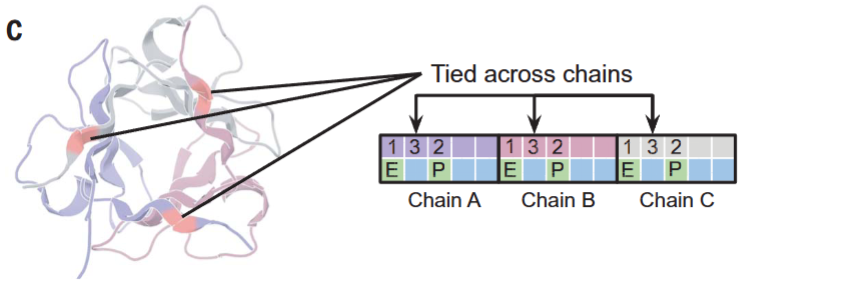
Tied residues (위치 결합):
Homo-oligomer나 repeat protein 설계 시, 대칭적으로 동등한 위치의 아미노산을 동일하게 강제하는 기능이다.
알고리즘:
- 결합된 위치들(예: Chain A의 position 1과 Chain B의 position 1)에 대해 각각 unnormalized probability를 예측
- 이 확률들을 평균(또는 가중 합)하여 단일 probability distribution 생성
- 이 분포에서 joint amino acid를 샘플링
Multistate design:
- 두 개 이상의 원하는 state를 인코딩하는 단일 서열 설계 가능
- 각 state에 대한 unnormalized probability를 예측 후 평균
- Positive/negative coefficient를 사용하여 특정 state를 upweight/downweight 가능 (explicit positive/negative sequence design)
5. Training with Backbone Noise

Insight:
- Gaussian noise (SD = 0.02 Å)를 backbone 좌표에 추가하여 학습하면:
- PDB 구조에 대한 sequence recovery: 감소 (50.8% → 47.9%)
- AlphaFold 모델에 대한 sequence recovery: 증가 (46.9% → 48.5%)
해석:
- 결정학적 refinement가 backbone 좌표에 아미노산 identity의 memory를 남길 수 있음
- Noise 추가로 이러한 local detail을 blur out하여 일반화 성능 향상
- Noised model은 전체적인 topological feature(예: overall polar-nonpolar sequence pattern)에 더 집중
의미:
- 0.3 Å noise로 학습한 모델: lDDT-Cα > 95 또는 > 90인 AlphaFold 예측을 생성하는 서열의 수가 2~3배 증가
- 더 높은 noise level: 덜 엄격한 lDDT cutoff에서 success rate 증가
- 원자 좌표가 정확히 알려지지 않은 실제 설계 상황에 더 robust
6. Sampling Temperature와 Sequence Diversity
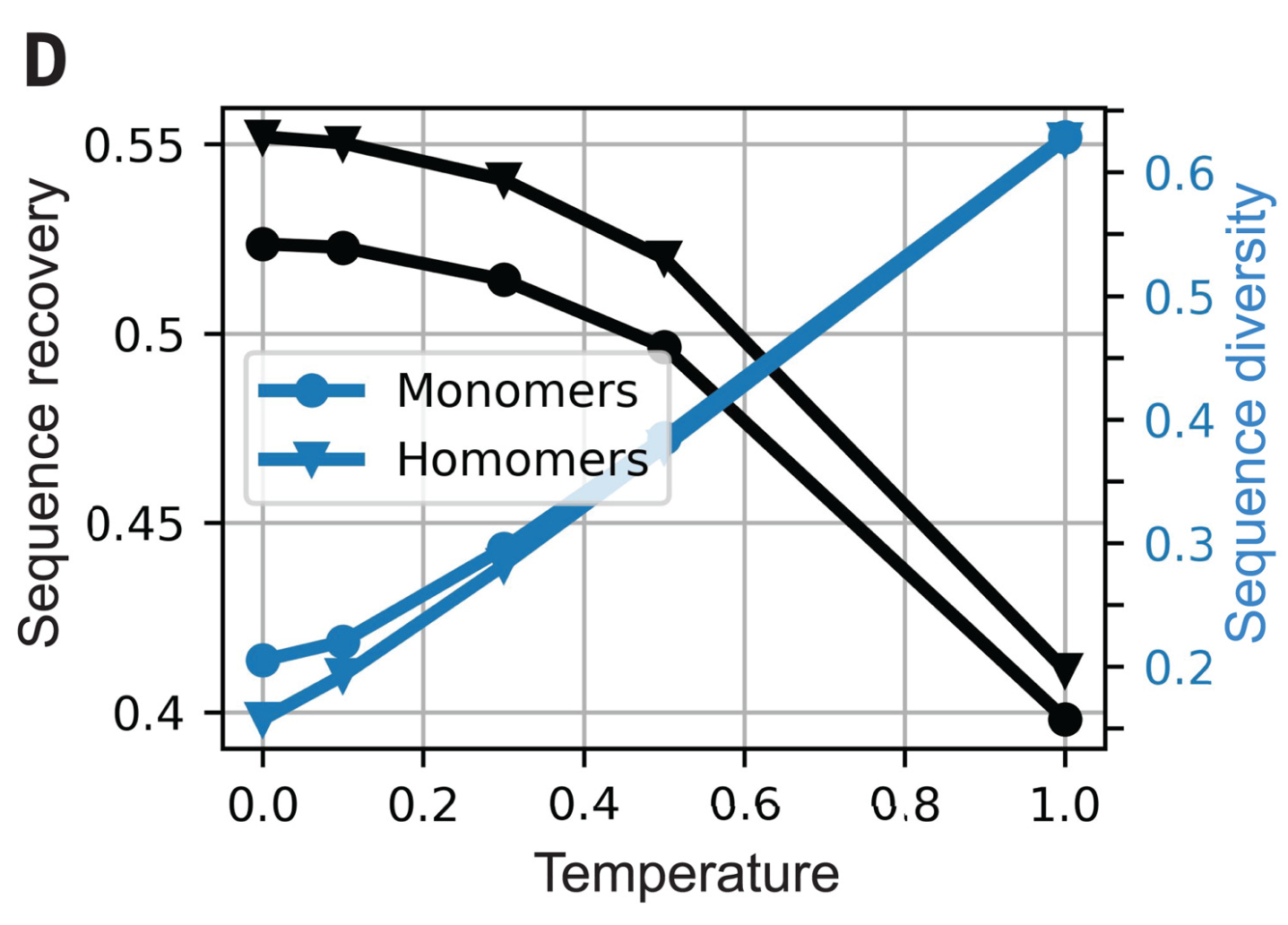
Observation:
- 높은 sampling temperature에서 inference 시 서열 다양성이 증가
- Sequence recovery는 약간만 감소
의미:
- 대부분의 단백질 설계 응용에서는 여러 후보 서열을 실험적으로 테스트하는 것이 바람직
- Temperature 조절로 다양한 서열 후보 생성 가능
7. Sequence Quality Metric

지표: ProteinMPNN에서 도출된 구조가 주어졌을 때 서열의 averaged log probability
용도:
- Native sequence recovery와 강하게 상관관계
- 다양한 temperature에서 생성된 서열들의 빠른 순위 매기기 가능
- 실험적 특성화를 위한 서열 선택에 활용
[5] Experimental Setup
1. Dataset Setup
(1) Protein Binder Design Benchmark
- PD-L1
- Insulin Receptor (InsulinR)
- IL-7Rα
- Angiopoietin-1 Receptor (Tie2)
- IL-2Rα
(생성)
- 각 타겟당 400개 backbone 생성
- 각 backbone당 4개 서열 (ProteinMPNN)
*평가 지표
- min inter-chain pAE ≤ 1.5
- binder pTM ≥ 0.8
- target-aligned binder Cα RMSD < 2.5 Å
→ Success 정의: 4개 ProteinMPNN 서열 중 최소 1개가 모든 조건 충족
(2) DNA Binder Design Benchmark
seq 1, 2, 3: 7RTE, 7N5U, 7M5W
(생성)
- 각 서열당 100개 구조 생성
- 각 backbone당 4개 서열 (LigandMPNN)
*평가 지표
DNA-aligned RMSD:
- Design과 AF3 prediction의 DNA phosphate 원자 정렬
- N/C terminus의 terminal loop 제외 후 protein Cα RMSD 계산
- < 1.5 Å: 우수
- 1.5-3.0 Å: 양호
- 3.0-5.0 Å: 통과
(3) Small Molecule Binder Design Benchmark
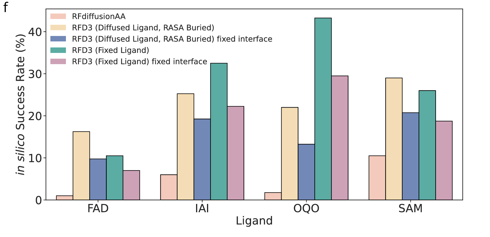
ligand: FAD, SAM, IAI, OQO
- 각 리간드당 400개 backbone 생성
- RFdiffusionAA의 published backbone 데이터와 비교
*평가 지표
Protein backbone RMSD ≤ 1.5 Å
Backbone-aligned ligand RMSD ≤ 5 Å
Interface min PAE ≤ 1.5
iPTM ≥ 0.8
(4) Enzyme Design Benchmark - AME
- 총 41개 active sites (PDB 출처)
- Residue island 개수: 1~7개
- 각 case당 backbone 생성 후 8개 서열 (LigandMPNN)
*평가 지표
Success 정의:
- Chai-1 (AlphaFold3의 오픈소스 재현) 예측 사용
- Motif backbone-aligned motif all-atom RMSD < 1.5 Å
- 8개 LigandMPNN 서열 중 최소 1개 통과 시 backbone success
2. Baseline model
| Model | Task | Details |
| RFdiffusion1 (RFD1) | Protein binder, Enzyme | noise scale 0으로 설정 |
| RFdiffusion2 (RFD2) | Enzyme (AME benchmark) | - |
| RFdiffusionAA | Small molecule binder | published backbone 사용 |
3. Inference time

- ~20초 (RFD3) vs ~200초 (RFD1/RFD2)
[6] Result
1. Unconditional Protein Generation
Designability:
- 100-200 길이 단백질 설계
- 98%의 설계가 AF3 예측 시 1.5 Å RMSD 이내로 fold
- 8개 ProteinMPNN 서열 중 최소 1개 기준

Diversity:
- 96개 생성물 (길이 100-250) 중 41개 cluster (TM-score 0.5 cutoff)

Sequence composition:
- ProteinMPNN 서열 분포와 유사하나 Alanine에 bias
- 원인 추정: 네트워크가 PDB 대비 compact globular fold 선호
2. Protein Binder Design

평균 unique successful clusters: RFD3 8.2 vs RFD1 1.4
논문 내용이 너무 많아서 파트를 좀 나눠야할 것 같다..(수정중)