0. Talktorials
모든 study 는 TeachOpenCADD 를 바탕으로 구성하였습니다.
T007 · Ligand-based screening: machine learning — TeachOpenCADD 0 documentation
Github:
1. Theory
앞선 T004 에서 ligand-based virtual screening 을 공부했었습니다. 그 때는 similarity search 방식을 중심으로 개념을 공부했는데, virtual screening 을 하는 방식에는 search 방식 말고도 여러가지가 있습니다. 헷갈리기 쉬우니 복습할 겸 virtual screening 부터 간단하게 정리해보겠습니다.
Virtual screening 은 원하는 protein target 에 activity 를 가지는 compound (ligand) 를 찾는 것입니다. 밑의 figure 는 일반적인 virtual screening 방식에 대한 모식도입니다.
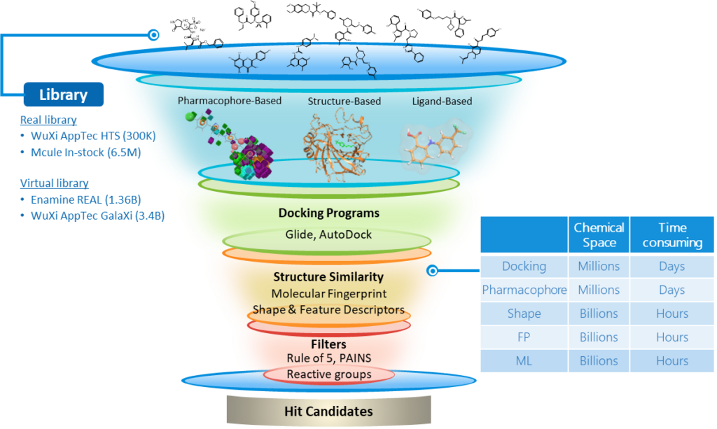
기본적으로 screening 하기 위한 chemical library 가 필요합니다. Docking programs, similarity search, filter 등 다양한 방식에서 연구자가 어떻게 설계하느냐 에 따라 virtual screening 방식은 자유롭게 이뤄질 수 있습니다.
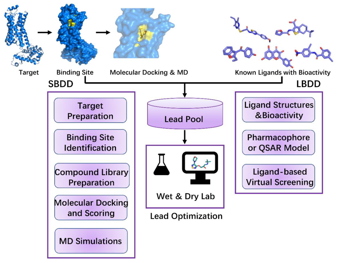
Screening 하는 방식은 target 구조 데이터 (PDB) 를 이용하는지의 여부에 따라 Structure-based (구조 데이터 존재 O), Ligand-based (구조 데이터 X) 로 나뉠 수 있습니다. 실험적으로 증명된 target protein 구조 (PDB) 를 이용한다면 사용하지 않을 때보다 target 특성에 맞게 모델이 학습할 수 있다고 예상되지만,

현재 PDB data set statistics 현황입니다. 2025년을 기준으로 235,666 data 가 존재합니다. 같은 target 이라도 binding form 이 다른 경우의 수를 생각하면 약 23만 개의 데이터는 매우 적은 수라고 생각이 됩니다. (요즘은 알파폴드 등 protein prediction 연구가 더 활발하게 이뤄지고 있기 때문에 이런 tool 들을 이용해서 data 를 준비하는 것도 하나의 방법입니다.) 내가 원하는 target 의 구조 데이터가 있다는 보장이 없기 때문에 ligand-based screening 하는 것도 고려하는 등 여러가지 가능성을 염두에 둘 수 있습니다.
T004 에서 배운 similarity search 방식은 target protein 의 구조 정보를 이용하지 않았기 때문에 ligand-based 입니다. T007 은 ML 을 이용하는 방식인데, input 하는 데이터에 target protein 의 구조 정보를 이용한 데이터를 넣지 않는다면 이 또한 ligand-based 로 virtual screening 을 진행했다고 말할 수 있습니다.
Virtual screening 의 대략적인 개념에 대해선 정리가 되었습니다. 이제 ligand-based virtual screening 에서의 ML 전략에 대해 알아보겠습니다. ML 을 제대로 screening 에서 적용시키기 위해서는 분자 large data, molecular encoding, label (hit 여부) 가 필요합니다. 그리고 screening 을 위한 ML 전략 또한 필요합니다.

1-1. Data preparation: Molecule encoding
분자를 ML에 사용하기 위해서는 feature 로 변환되어야 합니다. 분자를 feature 로 변환 시키는 대표적인 방법은 fingerprint 입니다. fingerprint 에 관한 내용은 T004 에서 자세하게 다뤘습니다.
T004 · Ligand-based screening: compound similarity
대표적으로는 MACCS 와 ECFP 등의 fingerprint 방식이 있습니다.
1-2. Machine learning (ML)
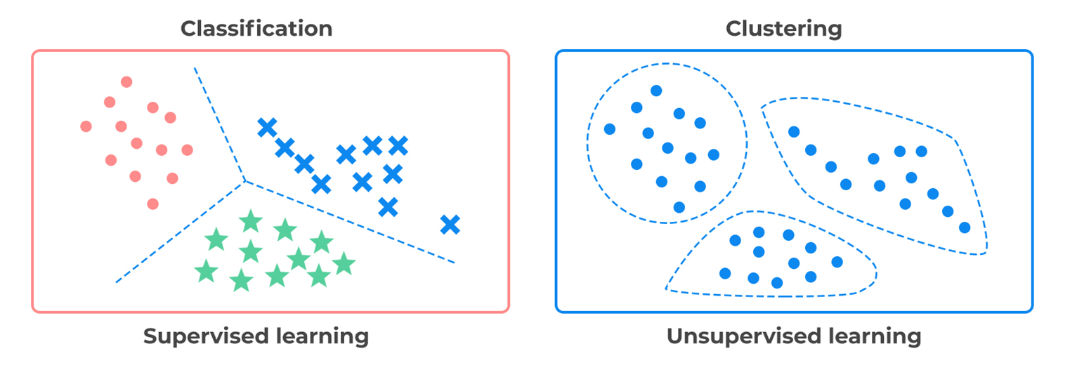
머신러닝은 보통 supervised learning 과 unsupervised learning 으로 분류됩니다. 두 방식의 가장 큰 차이점은 label 즉, 정답의 여부입니다. Supervised learning 은 예를 들어, 롯데 야구 팀이 경기에서 승리 or 패배 할 지에 대해 예측하는 문제나 현재 집 값이 1억이라면 5년 뒤에는 가격이 얼마일 지에 대한 구체적인 수치를 예측하는 문제 등 구체적인 답이 존재하는 문제를 해결하기 위한 ML 방식입니다.
반대로 unsupervised learning 은 label (정답) 이 없습니다. 정답이 없는데 뭘 예측하나에 대한 의문이 들 수 있지만, 데이터 분석할 때 이런 상황은 굉장히 많이 발생합니다. 예를 들어, 100 마리의 동물에 대한 데이터가 주어졌는데 데이터의 특성이나 분포를 분석하고 싶을 때 사용할 수 있습니다. 100 마리의 동물을 그룹별로 묶으려고 합니다. 각 동물에 그룹에 대한 label 이 존재하는 것이 아니라 동물의 특성을 반영해서 유사한 특성을 가진 동물끼리 같은 그룹으로 묶을 수 있습니다.
대표적으로 supervised learning 에는 Classification (분류) 와 Regression (회귀) 문제가 있고, unsupervised learning 에는 clustering (참고: T005 · Compound clustering) 이 있습니다.

위 그림은 scikit-learn 에서 제공하는 documentation 의 ML part 입니다.
다양한 알고리즘의 예시들이 제공되어 있어서 혹시 궁금하시다면 참고하시면 좋을 것 같습니다.
1-3.Model validation and evaluation
Validation strategy: K-fold cross validation

ML 에서 모델이 학습하고 난 뒤 잘 예측했는지 test 하는 것은 매우 중요합니다. 보통 ML 에서는 train data 와 test data 를 동일하게 하지 않습니다. 한 번 train 한 데이터를 재활용하여 또 test 를 위한 예측을 하게 되면 시험 문제의 정답을 알려주고 시험을 보게 하는 것과 마찬가지입니다. Test 결과에서는 모델의 성능이 좋음에도 불구하고 아직 보지 않은 새로운 data 에 대해서는 유의미한 예측을 하지 못할 겁니다. 이를 overfitting (과적합) 이라고 합니다. 과적합을 피하기 위해 ML 할 때는 주어진 data 를 train, test 로 미리 분리하고 학습을 진행시킵니다.
그런데 ML 에서는 이런 data 분할 말고도 고려해야 할 점이 하나 더 있습니다. 모델의 하이퍼파라미터인데, 이 하이퍼파라미터를 튜닝하기 위한 또 다른 data set 이 필요합니다. 보통 validation data 라고 부릅니다. 앞의 train, test 처럼 주어진 데이터에서 분할하면 되는데 이렇게 데이터를 train, test, valid 3분할 하게 되면 모델 학습에 사용할 수 있는 sample 의 크기가 매우 줄어들게 되고, 결과는 특정한 train, valid set pair 에 크게 의존할 수 있습니다.
이 문제를 해결하기 위한 Cross-validation 이라는 방법이 있습니다. 최종적으로 평가를 위해서 test set 은 여전히 분리되어 있어야 하지만, valid set 은 필요하지 않습니다.
Cross-validation 의 가장 기본적인 방식인 K-fold cross validation 방식을 설명드리겠습니다. K-fold cv 에서는 train set 을 k 개의 더 작은 set 로 나눕니다.

그림은 train set 을 5개의 fold 로 분리한 모습입니다. 여기서 fold 는 그냥 data set 과 동일한 의미라고 생각하시면 됩니다. (분리되어 있는 data set 이라서 fold) 매 학습마다 test set 을 다르게 해서 나머지 fold 로 학습을 진행합니다. Split 1 에서는 Fold 1 을 test set 으로, Split 2 에서는 Fold 2 를 test set 으로 ... Split 5 까지 진행합니다. model 은 그림과 같은 상황에서는 5번 돌아갑니다. 결과도 당연히 5개 나오게 됩니다. 단점은 계산량이 매우 많다는 것인데 그만큼 train 데이터를 기존의 방식보다는 더 많이 유지할 수 있다는 장점이 있습니다.
Performance measures
우선, 지금 소개할 performance measures 는 분류 모델에서 사용하는 지표입니다. 분류 모델의 성능을 시각화하는 방법이라고 생각하면 됩니다.
- Confusion matrix (혼동 행렬)
| What the model predicts | True active | True inactive |
| active | True Positive (TP) | False Positive (FP) |
| inactive | False Negative (FN) | True Negative (TN) |
- True Positive (TP)
- True Negative (TN)
- False Positive (FP)
- False Negative (FN)
단어가 계속 반복해서 쓰여서 헷갈릴 수 있는데 뒤에서 부터 해석하면 쉽습니다. Positive, Negative 는 모델이 예측한 값이고 True 랑 False 는 그 예측한 결과가 옳다, 틀리다 라는 것입니다.
True Positive (TP) 는 Positive 이므로 모델이 예를 들어, 어떤 한 분자가 active 하다 라고 예측하였는데 True ! 실제로도 active 한 것으로 정답을 맞힌 상황입니다.
그렇다면 True Negative (TN) 는 어떨까요? Negative 이므로 모델이 한 분자가 inactive 하다 라고 예측하였는데, True ! 실제로도 inactive 한 것입니다.
마지막으로 False Positive (FP) 는 뒤에서 부터 보면 Positive 이므로 모델이 어떤 분자를 active 라고 예측하였는데, False ! 실제로는 active 하지 않다는 것입니다. 즉, 실제로는 inactive 한 분자이기 때문에 모델 결과가 틀려서 False 라고 나타냅니다.
- Precision
- TPR = TP/(TP + FP)
- 모델이 양성(Positive) 이라고 예측한 데이터 중에서 실제로 그 데이터가 양성(Positive)인 비율
- Sensitivity, also true positive rate
- TPR = TP/(FN + TP)
- 실제로 양성(Positive) 인 데이터 중에서 모델이 얼마나 정확히 양성(Positive)를 예측했는가?
- Sensitivity 는 Recall 이라고도 부릅니다.
- Specificity, also true negative rate
- TNR = TN/(FP + TN)
- 실제로 음성(Negative)인 데이터 중에서 모델이 얼마나 정확히 음성(Negative)를 예측했는가?
- Accuracy, also the trueness
- ACC = (TP + TN)/(TP + TN + FP + FN)
- 전체 데이터 중에서 모델이 정확히 맞춘 비율
- 불균형한 data set 에서는 유용하지 않습니다. (예를 들어, 100명 중 99명은 암에 걸리지 않고 1명만 암환자라는 정보를 가진 데이터가 있을 때 모델이 100명 모두 암에 걸리지 않았다고 예측했을 때의 정확도는 99% 입니다. 실제로 암 환자를 찾아내지 못했음에도 정확도가 99% 라는 결과가 나오는 것입니다.)
- ROC-curve, receiver operating characteristic curve
- 분류 모델의 성능을 x축: 1-Specificity, y축: Sensitivity 로 나타낸 그래프
- 곡선이 왼쪽 위로 갈수록 좋은 성능
- AUC, the area under the ROC curve (AUC):
- ROC 곡선 아래 면적
- 모델이 임의의 Positive sample 을 Negative 보다 더 높게 분류할 확률
- 0과 1 사이의 값, 높을수록 분류 성능이 좋습니다.
2. Practical
GitHub - StructuralGenomicsConsortium/Target2035_Aircheck_Utils
Taret 2035 Aircheck DEL-ML example 라는 대회에서 제공한 basecode 입니다. 코드 설명에서는 예시는 예시일 뿐 이런 흐름으로 진행하지 말라고 되어 있지만, 일반적인 전략을 공부하기 좋은 코드 같아서 가져왔습니다. (대회는 target 이 어려워서 여러가지 아이디어가 필요한 상황입니다.)
Chemical fingerprint 에 기반한 ML 모델
import sys
sys.path.append("../ReadingParquetFiles") #Used to import module from different folder in the repository
from read_parquet_utils import read_parquet_file
from sklearn.model_selection import train_test_split
import numpy as np

data_file = "WDR91.parquet" #Change to the path to your file
df = read_parquet_file(data_file, columns = ['ECFP4', 'LABEL'])

x_train, x_test, y_train, y_test = train_test_split(df.ECFP4,
                                                    df.LABEL,
                                                    test_size=0.10,
                                                    random_state=42,
                                                    shuffle=True,
                                                    stratify=df.LABEL,)
x_train = np.stack(x_train)
x_test = np.stack(x_test)
y_train = y_train.to_numpy(dtype=int)
y_test = y_test.to_numpy(dtype=int)
code 에서 target 은 WDR91 이고, fingerprint 는 ECFP4 를 사용하였습니다. 모델 학습을 위해선 LABEL 이 필요하고 (hit 는 1, non-hit 는 0) 앞에서는 K-fold 중 한 fold 를 test set 으로 사용하였는데 이 코드에서는 전체 데이터에서 미리 10% 를 test set 으로 분리하고 K-fold 를 진행합니다. stratify=df.LABEL 는 LABEL data 의 class 비율을 유지하며 분할하겠다는 뜻입니다.
In an ideal case the external test set should not be selected at random from the existing training data, but here it is done for the sake of simplicity.
: 원래는 test set 은 기존 학습 데이터에서 무작위로 선택해서는 안 되지만, 여기서는 단순함을 위해 그렇게 했다고 설명합니다.
from sklearn.model_selection import StratifiedKFold
from sklearn.ensemble import RandomForestClassifier
from sklearn.metrics import precision_score, recall_score, f1_score,roc_auc_score

skf = StratifiedKFold(n_splits=5, shuffle = True, random_state=42)
for i, (train_index, test_index) in enumerate(skf.split(x_train, y_train)):
    model = RandomForestClassifier(n_estimators=10) #Reduced from the defult 100 to save time
    model.fit(x_train[train_index], y_train[train_index])
    y_score = model.predict_proba(x_train[test_index])[:,1]
    y_pred = model.predict(x_train[test_index])

    metrics = {"Precision": precision_score(y_train[test_index], y_pred, zero_division=0),
                "Recall": recall_score(y_train[test_index], y_pred),
                "F1-Score": f1_score(y_train[test_index], y_pred),
                "AUC-ROC": roc_auc_score(y_train[test_index], y_score)}

    print(f"Fold {i+1} Metrics:")
    for metric, value in metrics.items():
        print(f"{metric}: {value:.4f}")
    print("-" * 40)
정말로 다행인 점은 sklearn 에서는 K-fold 패키지를 제공해줍니다. (하나하나 코드를 짜지 않아도 함수로 쉽게 사용할 수 있다는 뜻) n_splits = 5 즉, 5-fold cross validation 입니다. 모델은 RandomForestClassifier 랜덤포레스트 모델을 사용했습니다. 결과는 예를 들어, 이런식으로 나옵니다.
Fold 1 Metrics:
Precision: 0.8816
Recall: 0.6326
F1-Score: 0.7367
AUC-ROC: 0.9515
----------------------------------------
Fold 2 Metrics:
Precision: 0.8807
Recall: 0.6342
F1-Score: 0.7374
AUC-ROC: 0.9511
----------------------------------------
Fold 3 Metrics:
Precision: 0.8825
Recall: 0.6207
F1-Score: 0.7288
AUC-ROC: 0.9487
----------------------------------------
...
model = RandomForestClassifier(n_estimators=10).fit(x_train, y_train)
y_score = model.predict_proba(x_test)[:,1]
y_pred = model.predict(x_test)

metrics = {"Precision": precision_score(y_test, y_pred, zero_division=0),
                "Recall": recall_score(y_test, y_pred),
                "F1-Score": f1_score(y_test, y_pred),
                "AUC-ROC": roc_auc_score(y_test, y_score)}

print(f"External test set Metrics:")
for metric, value in metrics.items():
        print(f"{metric}: {value:.4f}")
마지막으로 앞에서 분리해뒀던 test set 을 대상으로 예측 후 평가합니다.
(사실 여기서 흐름이 좀 이상한데, K-fold 의 모델들을 앙상블 하는 등.. 으로 진행하는 것이 좋긴합니다.)
import pickle
with open('Aircheck_WDR91_model.pkl', 'wb') as out:
    pickle.dump(model, out)
앞에서 사용했던 model 을 저장할 수 있습니다. ("model")
from sklearn.cluster import AgglomerativeClustering
from scipy.spatial.distance import pdist, squareform

top_5000 = np.argsort(y_score)[-1:-5001:-1]
cluster_fp = x_test[top_5000]
distance = pdist(cluster_fp != 0, metric = 'jaccard') #Turn the count ECFP4 into binary ECFP4
clustering_200 = AgglomerativeClustering(n_clusters=200,
                                    metric='precomputed',
                                    linkage='complete')
cluster_labels_200 = clustering_200.fit_predict(squareform(distance))
clustering_500 = AgglomerativeClustering(n_clusters=500,
                                    metric='precomputed',
                                    linkage='complete')
cluster_labels_500 = clustering_500.fit_predict(squareform(distance))
hits_200 = 0
hits_500 = 0
seen_cluster_200 = set()
seen_cluster_500 = set()
for sorted_index, original_index in enumerate(top_5000):
    if cluster_labels_200[sorted_index] not in seen_cluster_200:
        seen_cluster_200.add(cluster_labels_200[sorted_index])
        if y_test[original_index]:
            hits_200 += 1
    if cluster_labels_500[sorted_index] not in seen_cluster_500:
        seen_cluster_500.add(cluster_labels_500[sorted_index])
        if y_test[original_index]:
            hits_500 += 1
print(f"Numer or hits found in the selected 200 molecules: {hits_200}")
print(f"Numer or hits found in the selected 500 molecules: {hits_500}")
(code 작성자의 오타: Numer -> Number)
test set 에서 모델 예측 점수 (y_score) 를 기반으로 상위 5000 개의 sample 을 선택합니다. 이 상위 5000 개의 sample 의 ECFP4 를 추출하고 Jaccard 거리를 사용해서 similarity 계산을 합니다. clustering 을 진행하는데, 200개, 500개 cluster 로 나누고 200개 cluster 에서 발견된 hit 개수와 500개 cluster 에서 발견된 hit 개수를 각각 출력합니다.
정리하면, 5000 개의 sample 에서 cluster 를 200으로 설정하여 200개의 cluster 로 나누고 cluster 안에 hit 가 하나라도 있으면 count 가 되는 것입니다. 여러 개가 포함되어 있더라도 cluster 를 기준으로 1 count 가 되는 것입니다.
Numer or hits found in the selected 200 molecules: 132
Numer or hits found in the selected 500 molecules: 227
결과가 이렇게 나올 경우 200개의 cluster 에서 132개의 cluster 에서 hit 물질이 발견되었고 500개의 cluster 에서는 227개의 cluster 에서 hit 물질이 발견되었습니다. 이렇게 clustering 하고 평가하는 이유는 chemical 다양성을 위해서입니다.
T004 · Ligand-based screening: compound similarity 에서
Similar property principle (SPP) 및 Structure-activity relationship (SAR) 접근법은 structurally similar molecules 이 similar properties 을 가진다라고 가정합니다.
라고 설명하였습니다. 우리가 screening 을 진행하고 실제로 실험을 할 때는 테스트할 수 있는 분자의 수는 한정적입니다. 이 때, 비슷한 구조를 가진 compound 를 실험하는 것 보다는 신약개발 측면에서 다양한 구조의 compound 를 실험해보는 것이 더 중요할 것 같습니다.
Reference
- Virtual Screening & In Silico Drug Discovery - WuXi Biology
- scikit-learn: machine learning in Python — scikit-learn 1.6.1 documentation
- International journal of molecular sciences 23.21 (2022): 13568.
- PDB Statistics: Overall Growth
- Supervised Machine Learning, Unsupervised Machine Learning, and Deep Learning
- 3.1. Cross-validation: evaluating estimator performance — scikit-learn 1.6.1 documentation
- GitHub - StructuralGenomicsConsortium/Target2035_Aircheck_Utils
- 현재 관련 분야를 공부하고 있는 전문가가 아닌 학생이기 때문에 틀린 내용이 있을 수 있습니다.
- 오타와 틀린 부분을 댓글로 알려주시면 수정하도록 하겠습니다.
'Drug study > TeachOpenCADD' 카테고리의 다른 글
| T009 · Ligand-based pharmacophores (2) | 2025.07.07 |
|---|---|
| T008 · Protein data acquisition: Protein Data Bank (PDB) (4) | 2025.07.03 |
| T006 · Maximum common substructure (0) | 2025.05.07 |
| T005 · Compound clustering (0) | 2025.04.18 |
| T004 · Ligand-based screening: compound similarity (2) | 2025.04.16 |